Capabilities:
- Imaging UV and VIS fluorophores (eg Dapi, CFP, GFP, YFP, Alexa 488/568/647)
- Ideal for fixed specimens (oil objectives)
- Z-sectioning
- Motorized stage for tiled images
ON
Microscope
- Click VIS in the software
- Choose objective
- TL = transmitted light
- RL = fluorescence, choose colour under the reflect or tab or using the micro button
- When focused . . .
Software
Saving images
- Create or select a database
- Click save on the image and name
OFF
- Put the Argon laser into standby and turn off any lasers that won't be used by the next person, leaving on the ones indicated on the booking calendar
- Exit the software, Log Off and sign the logbook
- Turn off all the lasers in the Acquire>laser box and exit the software
- Shut down the computer
- Switches 3, 2, 1 and sign the logbook
-
Turn on the mercury lamp (if required)
-
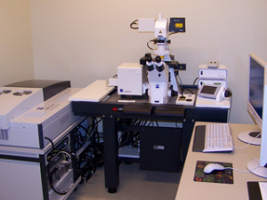
PC/system
-
Components
-
Logon to the local computer account
Double-click the 510 icon on the desktop, the LSM switchboard appears . . .

- Make sure Scan New Images is selected. ("Use Existing Images" is an off-line emulation mode)
- Click on Start Expert in the Switchboard.
And the software looks like this:

The objectives, fluorescent filters, condenser, neutral density filters, and field diaphragm on the Axio Observer stand are motorized and can be controlled in the software via the Acquire>Micro submenu or the LCD touchscreen. You may want to find and view your specimen under transmitted light or fluorescence, or both.
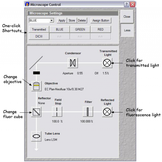
When you've located something you'd like to confocal, click the LSM button on the software panel.
Turn On the Lasers
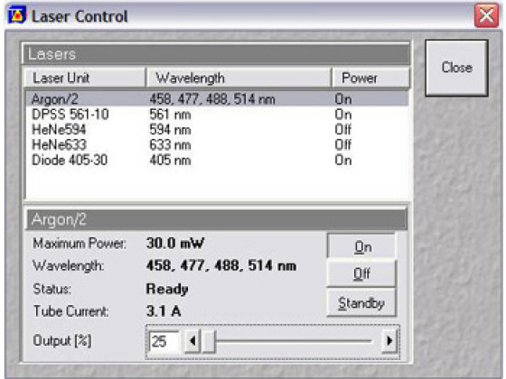
Select Acquire>Laser submenu will open the "Laser Control" window with a list of available lasers.
| Laser | Lines (nm) | Color of fluorophores | Examples of fluorophores |
| 405 Diode | 405 | Deep blue | DAPI |
| Argon | 458 477 488 514 | Green (Cyan and Yellow) | GFP, Alexa 488, FITC, CY2 |
| 561 Diode | 561 | Red | Alexa 568, TRITC, CY3 |
| 594 gas | 594 | Red | Alexa 594, texas red, mCherry |
| 633 gas | 633 | Far-red | Alexa 633, CY5 |
Turn on only the laser(s) you need to excite the fluorophores in your sample.
To turn on the Argon laser, click standby to warm it up. After the initial warm-up period, the on button will appear allowing the laser to be fully activated. Set the output intensity to an appropriate level - 40% is a good starting point.
To turn on any of the other lasers, simply click the appropriate "On" buttons - no warm-up is required for ignition.
We try to minimize the number of times a laser is turned on or off - if somebody will use the laser within 2 hours leave it on (Argon laser in standby). Check the reservation schedule to see the laser usage scheduled before and after your session. Turn off any lasers you don't need that may have been left on for you by the previous user, as long as anyone scheduled after you won't use them within 2 hours of your imaging session.
Choose a configuration
A filter configuration for the particular fluorophores you are using can be loaded via the "Configuration Control" window. Open it by selecting the Acquire>Config submenu.
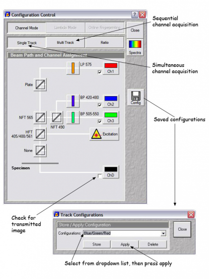
1. Single- or multi-track? Single Track mode is for single channel imaging or simultaneous excitation of multiple channels; in Multi Track mode the laser scans multiple channels sequentially, which can be useful when bleedthrough is a problem. Select whichever is appropriate for your imaging needs.
2. Apply preset configuration The saved configuration button on the right side of the "Configuration Control" window opens the "Track Configurations" window with many popular combinations.
Capture an image: Scan control
Acquire>Scan opens the "Scan Control" window - the main dialog box for acquiring images. There are several adjustments to make to get a good image. Each adjustment may effect the other settings so some interation in the process is required.
Adjustments under the channels tab . . .

1. Adjust % laser transmission(s) in the Excitation panel at the bottom of the window. Doing so sets the % laser power let through by the AOTF.
2. Set the pinhole diameter with the Pinhole slider scale. The smaller the pinhole, the thinner the optical slice will be and the less light will be collected. A pinhole set to 1 Airy unit (click the 1 button) will have optimal resolution. However, you will probably need to adjust this according to your sample's fluorescence, using larger Airy values for dim samples. For multi-fluorophore imaging, it is usually advisable to set the pinholes for each channel to produce equivalently thick optical slices.
3. Press "Find" to acquire a preliminary image using automatic setting of gain. An image display window will open and the output of the scan will be displayed. If you are performing multi-channel imaging, select Split XY button in the "Image" window's Display toolbar.

4. Click the Fast XY button and while the laser is scanning, use the XY Stage Controller and adjust the fine focus on the microscope body. Clicking "Stop" in the Scan Control window will turn off the Fast XY continuous scanning (minimize bleaching when you can).
The preliminary image, whether too dim or too bright, usually needs to be optimized. The PMTs need to be adjusted according to the fluorescence intensity of the sample.
5. Select each channel separately by clicking on the corresponding coloured button.
6. The range indicator display is helpful for setting the gain and offset. Select Palette in the image window's Select toolbar. From the Color Palette List, select "Range Indicator". In this palette, pixels with intensity of 0 are blue and pixels with intensity of 255 (for 8 bit images) are displayed red.
7. Start Fast XY and set the Detector Gain until no more than a few % of your stained areas has red pixels. Move the Amplifier Offset until the background is a mixture of blue and black pixels. (Always leave the amplifier gain as 1). Make these adjustments for each channel.
8. Reset the Palette to "No Palette".
Adjustments under the mode tab . . .
Most of these will be fine as the default values. Averaging is the most important thing to adjust.

512*512 pixels is good for most imaging, choose other pixel sizes in the "image size" sub-panel
Under Speed, the default scan speed (when not zoomed in) is 9. Reducing the scan speed can improve a noisy image; faster scan speeds are used to find regions of interest (like during the Fast XY function) or when photobleaching of the sample is a concern.
Under Pixel Depth, Scan Direction & Scan Average, select your images to be 8 bit (256 gray levels) or 12 bit (4096 gray levels). Select the Scan Direction to be unidirectional or bidirectional. Unidirectional is typically used, bidirectional scanning can be handy in live imaging since it cuts the scan time in half (but may require phase adjustment).
To set the averaging for your final image, choose between line averaging, using the mean intensity of 1,2,4,8, or 16 scans.
The amount of averaging necessary to obtain a good image depends on the signal to noise ratio of your sample image. Low contrast images will require more averaging but be aware that this could cause photobleaching. You can determine the amount of averaging necessary to yield the best image of your sample empirically. As a rough guide, averaging should be set to 100th the gain value, meaning most samples will require averaging of 4 or 8.
The zoom and scan field rotation can be set in the Zoom, Rotation, & Offset panel (Offset here refers to fine XY movement of the scan area). You may find it more convenient to use the crop function in the "Image" window -
Crop Your Image (optional)
This function is a true optical zoom performed upon image acquisition - the laser will scan a user-defined region of interest and display the scan data in the designated frame size (512x512, etc). It is a convenient way of setting the zoom, rotation and offset displayed under the Mode tab.
Press "Crop" from the Image window display toolbar. A crop box appears in the current image window, which can be moved, rotated and resized with the mouse.
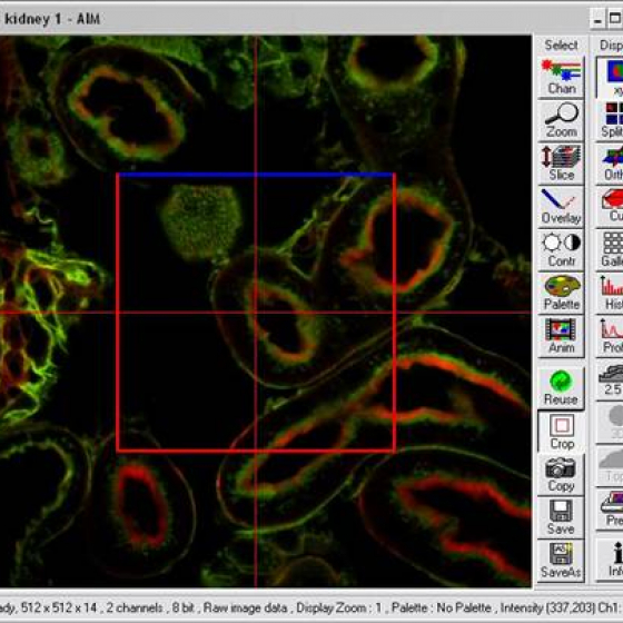
Pressing "single" will rescan with the modified zoom etc settings
(Pressing the "reset" button in the mode panel is useful for undoing all these changes, ready for the next sample.)
|
Images are overwritten so save as you go along
|
Z-sectioning
To collect a series of images at different points along the z-axis the settings can be inputted in two ways: Z Sectioning or Mark First/Last.
- Z-sectioning - takes x slices at a particular z interval
- Mark first/last - set the top and bottom of your sample and select either the interval or number of slices (the other is calculated for you)
Both of the methods described here assume that the user has optimized and set all imaging parameters, including pinhole size, detector gain/offset, scan time and averaging described above.
Mark First/Last Method
1. Select Z Stack at the top of the "Scan Control" window - doing this will activate the Z Settings panel.
2. Determine the start and end points of the Z stack. (Z sectioning is performed moving into the specimen, away from the coverslip.) To find the starting point for the Z stack perform a Fast XY scan and focus toward the coverslip (rotate fine focus knob toward you) until you reach the point at which you'd like to begin the Z stack. Stop the Fast XY scanning.
3. Click Mark First in the Mark First/Last tab in the Z Settings panel.
4.Start another Fast XY scan and turn the fine focus knob away from you focusing down through your specimen until you reach the point at which you'd like to end the Z stack. Stop the Fast XY scanning.
5. Click Mark Last to set the end point of the stack.
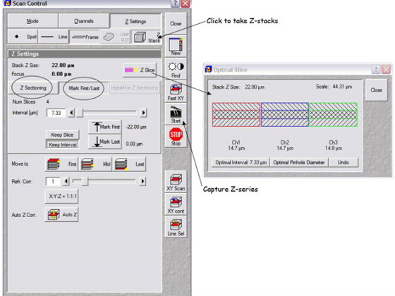
6. Assuming you have already adjusted your pinholes as described in "Acquire Menu: Collect An XY Section", look up the optimal z interval thickness by clicking Z Slice at the top of the Z Settings box. This will open the "Optimal Slice" window.
7. Optimal z interval thickness for the objective currently in use will be displayed in this window. Clicking Optimal Interval in the lower left corner of the window will set the z interval of your z stack to the recommended thickness.
8. Start will begin scanning of the z stack. Settings last entered in the Channels and Mode panels will be applied to this z stack collection.
9. The collected z stack is temporarily stored in the computer's memory. To permanently store the stack, use Save or Save As in the image display window to save it to a database.
Z Sectioning Method
1. This method assumes the user has prior knowledge of the specimen's thickness and/or is willing to guesstimate thickness. Select Z Stack at the top in the "Scan Control" window - doing this will activate the Z Settings panel.
2. Click on the Z Sectioning tab and select Keep Interval. This will keep the z slice size constant, even if you later decide to change the Num Slices or the upper and lower limits in your stack.
3.Type in the desired interval for your z stack in the Interval (um) field of the Z Sectioning tab. If necessary, look up the optimal z interval thickness by clicking Z Slice at the top of the Z Settings box. This will open the "Optimal Slice" window. Assuming you have already adjusted your pinholes as described in "Acquire Menu: Collect An XY Section", your optimal z interval thickness for the objective currently in use will be displayed in this window. Clicking Optimal Interval in the lower left corner of the window will set the z interval of your z stack to the recommended thickness.
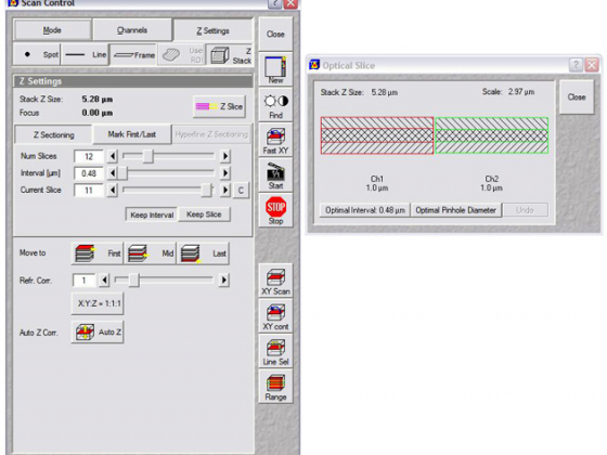
4. The Num Slices will be calculated automatically based on the chosen interval input.
5. Designate your current focal position (if you're in focus, you're probably somewhere near the middle of the specimen) in the Current Slice field.
6. Clicking Start will begin scanning of the z stack. Settings last entered in the Channels and Mode panels will be used to collect this z stack collection.
7. The collected z stack is temporarily stored in the computer's memory. To permanently store the stack, use Save or Save As in the image display window to save it to a database.
The Time Series is a versatile software function that is useful in a variety of situations - from collecting single confocal images or entire z stacks over time to more sophisticated applications such as FRAP. If desired, a delay between the beginning of one scan process to the beginning of the next can be set. It is important to note that Time Series works at only one location on the slide. To apply the Time Series function to multiple stage locations, you will have to use the Multitime macro.
The following instructions are for applying a basic Time Series. It is assumed that the user has optimized and set all imaging parameters beforehand (pinhole size, detector gain/offset, scan time, averaging, and if desired, z stack). Refer to previous sections for more details on adjusting these settings.
1. Select the Acquire>Time Series submenu.
2. In the Start Series panel, choose between a Manual start or a timed start via Time. Most users want a manual start. If a timed start is desired, enter a start time in the Time (h:m:s) field. The time series will start when the set time is reached according to the computer's clock.
3. In the End Series panel, enter the number of time points desired in the Number field if a Manual end is selected. For a timed end point, depress Time and enter the end time in the Time (h:m:s) field.
In determining an experiment's length and the number of time points needed it is important to consider the scan time and averaging settings (see the Speed section of the Mode panel in "Scan Control"). Both parameters influence how long it takes the laser to clear the scan field and thereby define the minimum time between time points.
4. The next panel you encounter will be either Time Interval or Time Delay, depending on the settings of your Time Series register (see Options--> Settings). Time Delay is defined as the end of one scan process to the beginning of the next, while Time Interval is the time between the beginning of one scan process to the beginning of the next. Either panel, Time Interval or Time Delay, permits time series scan parameters to be activated or changed from experiment to experiment.
You may load & Apply previously saved time series settings using the pulldown menu in either of these panels. Or you may choose to manually enter scan parameters into the Time and Unit fields. If you foresee performing other experiments with identical time scan settings, you should Store your manually entered settings to the dropdown list for easy reference in the future.
5. Click Start T in the right-hand side of the "Time Series" window to start your time series.
6. The collected time series is temporarily stored in the computer's memory. To permanently store the series, use Save or Save As in the image display window to save it to a database.
Remove your sample from the stage and clean any oil objectives you used. Please let us know of any problems, the Report Problem form at http://microscopy.duke.edu/feedback is quick to use.
Check the on-line reservation schedule to see if/when the next reservation is scheduled:
If someone else is scheduled to use the microscope within 2 hours...
- Put the Argon laser into standby and turn off any lasers that won't be used by the next person, leaving on hte ones indicated on the booking calendar
- Exit the software
- Record your use of the system using the CoreResearch booking system
- Select the "Log Off" command from the Start menu of the desktop and leave the system on.
If you are the last scheduled session of the day or for more than 2 hours...
- Turn off all the lasers in the Acquire>laser box and exit the software
- Record your use of the system using the CoreResearch booking system
- Select "Shut down computer" command in the Start menu of the desktop. The computer and monitors will power down automatically.
- Turn off the Components switch
- Turn of the PC/system switch
- Turn of the arc lamp