Zeiss 880 Inverted Confocal Manual

Power Up

1. Turn on the fluorescence lamp (#1) (if you need to see fluorescence down the eyepieces)
2. Turn on the main power switch (#2)
3. OPTIONAL For Live Imaging. Turn on power strip to the right of the system (#3)
4. Turn on systems/PC (#4)
5. Turn on components (#5)
6. Start the PC (#6)

Logging In and Starting the Software

1. Select the "LMCFuser" account and enter the password
2. Double-click the ZEN Black icon on the desktop and choose "Start System" when the boot status window pops up

Go to the Locate tab and choose to view your sample with transmitted light or fluorescence.

To turn off the transmitted light choose “Off” or close the shutter, similarly, to turn off the fluorescence light choose reflected light “Off” or close the shutter. Alternatively, choose “All Off” to turn off the path currently active.

Go to the Acquisition tab and check the 'Show all Tools' options for access to most acquisition options

Load Setup

LMCF has made multiple multi-track (sequential) scanning configurations. We strongly suggest that you load one of these as a starting point. Most of the setups are line-switching for speedier operation and less mechanical failure thanks to no mechanical movement in the scanning module. 

Smart Setup

If you do want to follow the 'Smart Setup' wizard, please choose the ‘Smartest (line)’ configuration when possible. Have in mind the Smart Setup path does NOT necessarily assign the fluorophores chosen to the optimal detector for their emission wavelength. Specifically, fluorophores with wavelengths in the middle of the visible light spectrum may NOT be assigned to the higher sensitivity GaAsP detector (ChS1).

Reuse a Previous Configuration

Open an image (in .czi format) and click ‘Reuse’ button at the lower middle of ZEN window to load the previous setup. Please remember configurations from images can only be reused in the microscope in which they were originally acquired as every microscope (even of the same model) are slightly different.

Manual Setup

You can manually change the excitation laser lines, emission bands, assigned detector, dichroics etc in the Imaging Setup menu.

• The MBS (Main Beam Splitter = dichroic) needs to match the lasers used in the visible and 405 light paths)
• One track for simultaneous imaging of the channels, more than one track for sequential scanning
• For multi-track: Frame switching should be used if different dichroics, pinholes or overlapping emission bands are required. Line switching is more convenient and possible when only electronic things change between tracks (eg AOTF control of excitation, which detector is active)
• Ch1 and Ch2 are standard alkali PMTs, ChS1 is an array of 32 high-sensitivity GaAsP PMTs.  This can be used as up to 8 channels in Channel mode. But they have to have the same master gain at any time, in which case you need to adjust laser power for proper image intensity.

In Live view, adjust the Z position with the fine focus knob to choose a plane of interest. If you are taking a Z-stack choose the brightest plane to adjust the settings. 

If Zoom is desired, either manually set the Zoom factor in the 'scan area' options under Acquisition Mode or use the Crop function under the image and resize the box.

Adjust the laser power so you have a reasonable excitation. The lowest value that will produce a bright image is best to minimize fluorophore saturation and photodamage.

Adjust the pinhole size so a suitable optical slice is obtained. There is a trade-off between resolution and brightness. A pinhole size of one Airy unit essentially gives you the best compromise between resolution and brightness. Opening it slightly from there will allow you to collect more signal. For multi-track scanning, set the pinhole in the channel with the longest wavelength. The other channels will automatically match the section thickness.

Adjust the master gain (signal amplification at the detectors) and digital offset (noise floor) for each channel. Selecting the range indicator is helpful when doing this. In this mode saturated pixels are highlighted red and 0 intensity blue. An image with few red pixels and about 90% of the empty area of the sample in blue is often a good level to aim for. A master gain around 800 volts and digital offset no less than -2 (when 8-bit images are acquired) are usually good. Remember, higher gain produces more noise in the image.

Image size (sampling rate) – the number of pixels in the image can be entered or selected from presets. The optimal button selects the pixel numbers for a particular objective, wavelength and zoom. This will give you a digital sampling rate adequate to fully sample the optical resolution. In most cases 1024x1024 is necessary and good for publication.

Scan speed and averaging – slower scan speed and averaging improves the signal to noise ratio (SNR). You need to choose a good balance for image quality and acquisition speed.

Click the disk icon beneath the open images icons or save as… to save the selected image(s) as .czi files. You will need to save as you go otherwise images might be overwritten by subsequent scans. Images in .czi format can be opened by freely available software such as ZEN lite, and FIJI.

Z-stack

Check the Z-stack option, go live and with the fine knob find the top (set first) and bottom (set last) of the specimen. Select optimal slice interval and then 'start experiment'.

Time Series

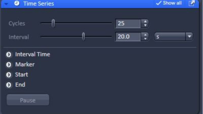
Check the Time Series box underneath the Z-series box. Choose the number of time points and the interval between them. Press 'start experiment'.

Tile Scan

• Set up tile region:
  • Centered grid: choose number of tiles in horizontal and vertical directions
  • Bounding grid: choose at least two positions on the sample and ‘Add’ (mark) them in the program. ZEN will draw a rectangle around those two diagonal marks. Add more marks outside the region when needed to expand the rectangle so that it covers the whole sample area you want to image.
  • Convex hull: works like bounding grid, but marked area is not a rectangle
• Overlap: 10-15% between image tiles as a starting point.
• Bi-directional: image tiles are captured in a meandering way, which is preferred.
• Online stitching: tiles are stitched into a single image immediately after all image tiles are acquired. Alternative to online stitching, image tiles can also be stitched at a later time (Processing tab --> stitch).
• Press ‘Start Experiment’

Coupling a tile scan to a Z-stack will result in better stitching in circumstances when your sample is in different planes (e.g large sections of tissue, cells in matrigel, etc)

1. Once you finish acquiring and savings your images center the stage, lower the objective all the way, and switch to the lowest magnification objective.

Live Imaging Controls                                  

At the end of your live imaging session, set the temperature in the H Unit XL close to room temperature (25°C). To avoid damage to the system, WAIT until the temperature has reached the set point of 25°C to uncheck the controls. 

2. Check the LSM 880 schedule in CR@D.

• If someone has signed up within 2 hours - Turn the Argon laser to “Standby” in the software
• If someone has signed up 2+ hours after you, or you are the last person for the day- Turn off the system following the next steps. 

4. First, please turn off all the lasers in the software, and ensure the Live Imaging Controls are off following the directions above as necessary.
5. Turn off the PC (#6).
6. ONLY when the noise from the Argon laser cooling fan has stopped, turn off in reverse order (#5-#1).