Capabilities:
- Widefield fluorescence imaging
- Motorized stage for tiling/stitching
- Transmitted light images - brightfield, DIC
- Colour camera for IHC (e.g. H&E staining)
- Z-stacks
- Apotome for optical sectioning
- (Optional) HXP 120V for fluorescent samples
- Power strip
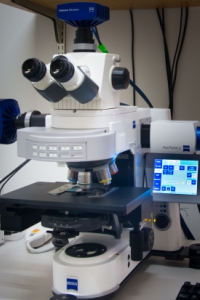
- Microscope
- (Optional) Apo-Tome
- Computer- Log-in to the computer, Open the program: ZEN
The fluorescent lamp should always be first-on. This prevents any electrical surges caused by ignition that damages other equipment on the same circuit.
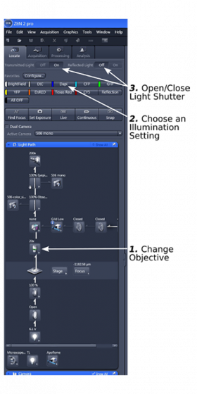
Lower down the stage a bit to avoid scratching of the objective when loading slides; Push in the light path switching slider; Load the sample; The ZEN opens to 'Locate' tab.
Step 1: Choose an objective from the drop-down list. Position the sample right under the objective.
Be alert that most of the objectives on the microscope have very short working distances. Avoid crashing of the objective with the sample. It is a good idea that you start with the 5x objective.
Step 2: Choose an illumination type from the presettings and focus on/view the sample under the eyepieces. The light shutter can be opened or closed (step 3). It is advised that a fluorescent sample should be illuminated as little as possible.
| Position | Magnification | NA | Dry/Oil | Working Distance |
| 1 | 5X | 0.16 | Dry | 12.1 mm |
| 2 | 10X | 0.45 | Dry | 2.0 mm |
| 3 | 20X | 0.80 | Dry | 0.55 mm |
| 4 | 40X | 0.90 | Dry | 0.41 mm |
| 5 | 63X | 1.4 | Oil | 0.19 mm |
| 6 | 100X | 1.4 | Oil | 0.17 mm |
Note: although the TRITC and the Texas Red filters are both good for red dyes, the TRITC filter is best for TRITC, DsRED, Alexa Fluor 555, Alexa Fluor 568, Cy3, etc.; Texas Red filter fits best Texas Red, mCherry, Alaxa Fluor 594, and so on.
Click the 'Acquisition' tab to open the acquisition module
Part 1: Fluorescent samples
1. Start with 'Experiment Manager' to choose a presetting from the dropdown list (step 1).
Note: All presettings for fluorescent samples are for 4-color channels (blue, green, red, and far red), but they are also good for 3-, 2-, or 1-color samples.
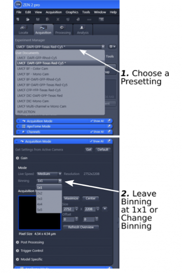
2. Open 'Acquisition Mode' (step 2) to select camera binning. Most of the time leave binning at '1x1'. If you wish to increase the sensitivity of the camera, you can choose other binning options, but at the cost of lower resolution in the image.
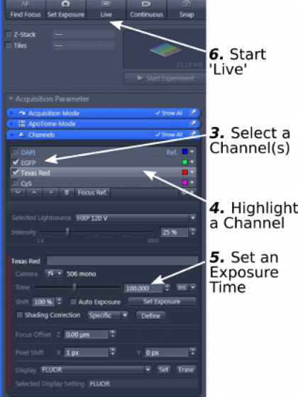
3. Open the 'Channels' window and select the fluorescent channels you need to image (step 3)
4. Highlight a channel (step 4) and set a short exposure time (for example 200ms) (step 5)
5. Start 'Live'(step 6). A live image will show up.
6. Click 'Min/Max' (step 7) above the histogram to automatically adjust the contrast of the image
7. Hover the mouse pointer over your interested objects and read the intensity ('Pixel Value') (step 8); Read also the intensity of a clean background. The intensity difference shall be at least 3 times for a publication quality image. If it is less than 3 times, try to increase the exposure time and/or light source intensity, but watch out for highlight clipping (histogram touches the right boundary) and photobleaching of the sample. Please don't use 'Auto Exposure' or 'Set Exposure' function, especially if you are comparing intensities from different samples.

8. Repeat step 4-7 for other channels
9. One click of 'Snap' to take the images for all selected channels
10. All acquired images will be lined up on the right side of the ZEN window.
11. After acquisition, a merged image shows up. Individual channels will be displayed by clicking 'Split' at the left side of the images.
12. Save images as '.czi' format file in one of the 'User DATA Drives'
Part 2: Color samples
1. Start with 'Experiment Manager' and choose 'LMCF BF-Color Cam' (step 1)
2. Open the 'Channels' window (step 2)
3. Uncheck 'Shading Correction' (step 3) if it is selected when you start your session
4. Start 'live' (step 4). A live image will show up.
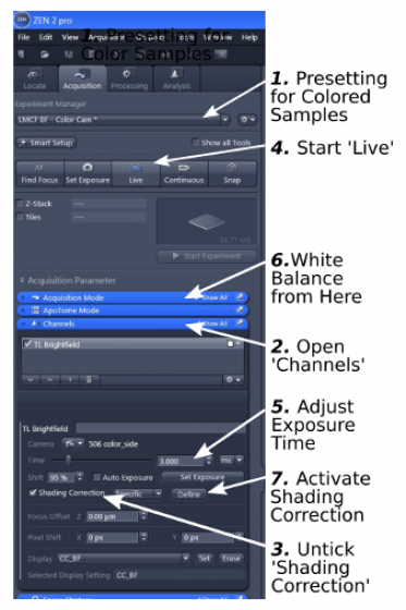
5. Click 'Min/Max' above the histogram to automatically adjust the contrast of the image
6. Find a good exposure time (step 5) so that the histogram will extend in the histogram box, but make sure that the right end of the histogram does not touch the right boundary of the box, an indication of overexposure.
7. White balance: back to 'Acquisition Mode' (step 6), click 'pick...' to change the mouse cursor into an 'eye dropper', use the 'eye dropper' to click in a completely blank area in the live image, which sets the background color to white.
8. Shading correction: move the stage and find a clean blank area in the sample, de-focus a little if the area still contains tiny objects, click 'Define' (step 7) in 'Channels' to generate a shading correction reference. 'Shading Correction' will be ticked and the function be activated.
9. 'Snap' the images and save them in '.czi' format in one of the user data drives
1. Contrast of image: For each fluorescent channel (step 1) separately, the white and the black points of the histogram can be adjusted by dragging the wedges or typing a number in the box for 'Black' or 'White' (step 2) to produce better contrast of the image.
2. Annotation: The most common annotation is to stamp a scale bar on the image by clicking the 'Scale Bar' icon under 'Graphics' (step 3). The bar can be edited for size, color, position in the image, etc. (step 4).

Click "Processing' to open the functional module
1. The most recently used 5 functions show up in the 'Method'. More processing functions can be found in the lower part of the 'Method' window.
2. 'Image Export' will save the image in a format that other graphic software can open.
A. In 'Input' window, choose the image to be exported.
B. In 'Parameters' window, you can choose a presetting 'Export Fluorescent Image to 'D Drive' for fluorescent images, or 'Export Color Image to 'D Drive' for images taken with the color camera.
C. If you choose to set up your own parameters, we recommend that you export the images in TIFF without downsizing (100% original size), conversion to 8-bit, nor any lossy compression. For fluorescent images, exporting the 'Original Data' is useful for future analysis. Applying 'Display Curve and Channel Color' and 'Burn-in Graphics' will retain the modified contrast in display as well as the scale bar in the images.
D. Click 'Apply'.
3. Images can also be processed in 'Batch' if they have been saved first.
Lower down the stage; Check the online booking calendar to determine whether you should turn off the system or leave it on for the next user
1. When to leave the system on:
A. You have used the fluorescent light source and another user will need to use the fluorescent light in one hour, leave the fluorescent light and the system on; If no other users will need the fluorescent light, you can turn the light off, but leave other things on.
B. You don't use the fluorescent light and the next user will not need to use the fluorescent light in one hour, leave the system on.
2. When to turn off the system:
A. You don't use the fluorescent light and the next user will need to use the fluorescent light.
B. Nobody will use the microscope in one hour or you are the last user for the day.
3. System is turned off in the backward order:
A. Computer (#5 from the start menu)
B. Apo-Tome (switch #4 if you have used it; don't forget to return the Apo-Tome module to resting position)
C. Microscope (switch #3)
D. Power switch (switch #2)
E. Fluorescent light (switch #1, if you have used it)
Note: Once the fluorescent light source is turned off, DO NOT turn it on again in 30 minutes.
1. Tiling and stitching:
This function is to generate a high-resolution image that covers a large area. It works for both color and fluorescently-labeled samples. The following steps are for color samples.
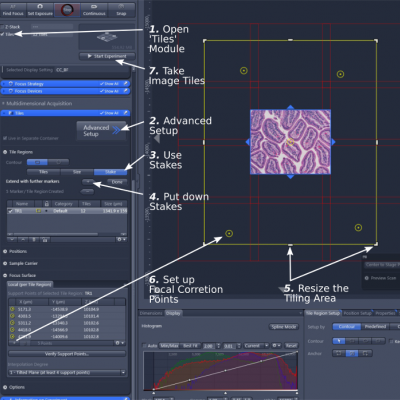
A. Set up exposure, white balance, and shading correction (see procedures above)
B. Open the functional module 'Tiles' (step 1)
C. Open 'Advanced Setup' (step 2)
D. Set imaging area: In 'Tile Regions', highlight 'Stake' (step 3). Move the stage manually or double click in the image display panel and add stakes (step 4). You need to put at least two virtual 'stakes' on your sample for the software to mark a rectangular area around them. The area that the future final image covers will show up as tiles in the display panel. Moving the stage to a position outside the current boundary, and adding 'stake' again will update and expand the boundary. You can also drag the yellow line with the mouse to resize the area (expanding or trimming) (step 5).
E. Set focus correction points: This function allows the program to use focuses set by the user. Open 'Focus Surface', move the stage to a position, focus, and add ('+') the information (X,Y, and Z parameters) in memory (step 6). Repeat adding focus points. For image tiles between the focus points, the software will determine the focuses based on those of the surrounding tiles.
F. Click 'Start' to acquire the image tiles
G. Stitch the image tiles into a single image: open 'Processing' and select 'Stitching'; In 'Input', choose the image tiles you wish to stitch; In 'Parameters', choose 'New Output' and 'Fuse Tiles'
H. Click 'Apply' to start the stitching process. The stitched image will be displayed as a separate image and should be saved in .czi format.
Please note: the stitched image can be big in file size that often times exceeds 4GB, which is the size limit TIFF format can handle. When exporting those images in ZEN as TIFF or JPEG files, the program may report various errors. If that happens, export the images instead as 'BigTIFF' format, then open them in 'Irfanview' (free program already installed on the Axio Imager computer). In Irfanview, further save the files as JPEG or other format.
2. ApoTome:
This Zeiss technology uses structured illumination and computation to cut off scattered light from out-of-focus planes, which generates images with enhanced contrast and higher resolution. This technology only works with fluorescent samples.
A. Push in the ApoTome.2 module. There is a beep when the module is engaged.
B. Choose number of frames. Usually 5 image frames are taken.
C. Image as usual (See procedure above). However, in comparison to regular imaging, the exposure time/illumination intensity need to be increased by several folds. Also, make sure the grids are in focus.
D. Processing of the ApoTome images: open the tab 'ApoTome' below the display panel, click 'Create image' to generate a processed image.
E. When finishing session, please disengage the ApoTome.2 by very carefully pulling it out until you feel a notch.
3. Reduction of file size:
The AxioCam 506 cameras on the microscope are of high resolution, which translates to bigger files. Although we suggest that you take advantage of the high resolution, there are still chances that you need smaller files. The following are some of the ways to achieve this goal:
A. Before acquisition, bin pixels of camera (under 'Acquisition Mode'). This reduces the resolution of the image.
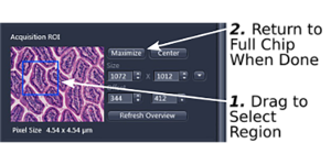
B. Before acquisition, using only a portion of the camera to cover a smaller area (under 'Acquisition Mode') (step 1). Please return to maximal image size when you are done (step 2).
C. After acquisition, 'Resample' the image (under 'Processing') by putting in a 'Scaling' factor that is smaller than 1. This process reduces the resolution of the image.
D. After acquisition, draw a 'region of interest' in the image using the ROI tool under 'Graphics'. Right-click on the marked area and 'Create Subset Images from region of interest' to duplicate the selected image within the region of interest.
E. In 'Image Export', in the case of exporting particularly large images, (a) set a percentage under 'Resize'; or (b) export image in 'JPEG' format. Both processes reduce resolution of the image.