This user's guide is complementary to the original manual that describes the imaging procedure with MetaMorph. For multidimentional image acquisition, please refer to the original user's manual.
Before turning on the system, please make sure a proper sample adapter is already installed on the stage. If not, install it before powering on the system. If the microscope is already on, switch off the microscope (#6) before installing the sample adapter. Otherwise the motorized stage may be damaged.
- (Optional) Fluorescent X-cite light (#1) if fluorescent samples are imaged; otherwise leave if off
- Power strip on the shelf (#2)
- Computer (#3) and log in as 'lmcfuser'
- (Optional) Evolve EMCCD camera to the left of the microscope (#5) if you are going to use it; otherwise leave it off
- Microscope (#6)
- (Optional) CoolSNAP HQ2 camera to the right of the microscope (#7) if you are going to use it; otherwise leave if off
- Open ZEN 2.3 Pro
There are 4 stage inserts for holding different samples - a heated insert for a 35 mm glass-bottomed dish or a chambered glass coverslip, an insert for multi-well plates, a universal frame for holding a slide or a dish, and another universal frame with clamps for holding slides.
Nearly everything on the microscope is motorized so can be controlled either on the LCD touchscreen or through ZEN.
Objectives
| Mag | NA | Oil? | DIC? |
|---|---|---|---|
| 2.5x | 0.075 | NO | NO |
| 5x | 0.16 | NO | NO |
| 10x | 0.30 | NO | Ph1 |
| 20x | 0.8 | NO | DICII |
| 40x | 0.75 | NO | DICII |
| 100x | 1.4 | Yes | DICIII |
1. ZEN 2.3 Pro opens to 'Locate' page by default. Lower down the objective a bit before loading the sample; Position the sample right above the objective
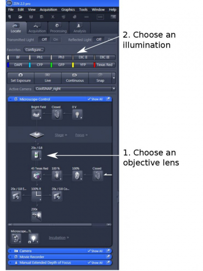
2. Choose an objective lens from the drop-down list in the program (step 1), on the touch pad, or from the objective field on the right side of ZEN
3. Choose an illumination (step 2). The quick access buttons are available for BF, PH1, DICII, DICIII, DAPI, Cy5 (Far Red) , GFP. YFP, and Texas Red. The CFP and Cy7 (near-infrared) filter cubes are not installed, but are available upon request.
4. Coarse/fine focus knobs are on the microscope. X-Y stage movement is through the rotary controller. Focus on the sample; Change to a different objective if it is desired and fine tuning of the focus may be needed.
Basic Acquisition (Single Field):
1. Load one of the two pre-settings dependent on which camera will be used (step 2). The higher sensitivity Evolve EMCCD is attached to the left of the microscope and the CoolSNAP ES2 to the right.
2. Open 'Channels' and tick all the channels you want to acquire images from (step 3)
3. Finding a good exposure for each channel, but don't use 'Auto Exposure' or 'Set Exposure' function
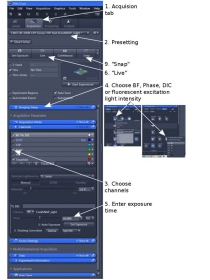
- For 'BF, Ph, DIC' channel:
(1) You need to use the objective-matching illumination (BF, Phase contrast, DIC) under 'Imaging Setup' (step 4).
(2) Enter an exposure 'Time' and/or light 'Intensity' (step 5), start 'Live' (step 6); A live image will show.
(3) Adjust the exposure time and/or light intensity, so that the histogram of the image (showing under the live image, step 7) will extend to the right of the histogram box, but don't let the intensity of the brightest pixels exceed about 70% of maximum
(4) Optional - 'Shading Correction': move to an empty and clean area, still in live mode, click 'Define'. The system will acquire a shading correction reference image and activate the function.
- For fluorescent channels:
(1) Choose an exposure 'Time' (step 5) and/or an excitation light intensity (under 'Imaging Setup', step 4) and start 'Live' (step 6).
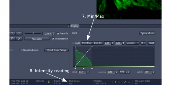
(2) Click 'Min/Max' or tick 'auto' in 'Display' section right below the image (step 7). This will adjust the contrast of the image for easy viewing of it.
(3) Hover the mouse pointer over your interested structure and read the intensity value at near the bottom of the ZEN Window ('Pixel Value", step 8), and also read the intensity of a clean background. Adjust exposure time and/or excitation light intensity so that pixel value of the interested structure is 3 times or more over that of the background.
4. Click 'Snap' (step 9) to take images from all selected channels, and a merged image will be displayed. Individual channels can be separately displayed by click "Split"
5. Save images in ".czi" format
Tile-scanning:
Tiling and stitching is used to generate a high-resolution image that covers an larger area out of multiple continuous fields.
Part One: Quick tile image acquisition
This function is built in 'Snap' button. You can choose to 'Snap' single images (see above), or 2x2, 3x3, 4x4, 5x5 image tiles around the current position.
Part Two: Tile-scanning from a slide
Tick 'Tiles' to activate the function (step 1), determine a good exposure for each channel (see above) before proceeding to the next steps
1. Under 'Tiles' section, click 'Advanced Setup' (step 2). The display window is divided into two parts for a virtual stage and a live image of the highlighted channel.
2. 'Tile Regions' set up: To mark the area to be imaged
(1). In 'Tile Regions', choose a 'Contour' and highlight 'Stake' (step 3)
(2). Move the sample stage and mark the stakes with the '+' sign (step 4). There need at least two diagonally positioned virtual 'stakes'. The system will draw a rectangle or a circle around them.
(3). The yellow line-enclosed area marks the desired area, while the red-lines tiles will be the actual images to be taken. Check all areas outside the red tiles to make sure the desired imaging area is completely within the red tile-marked boundaries. Otherwise, keep adding (the '+' sign) or drag the yellow line outwards (step 5). The area will update and expand. To trim or reduce an area, drag the yellow line inwards
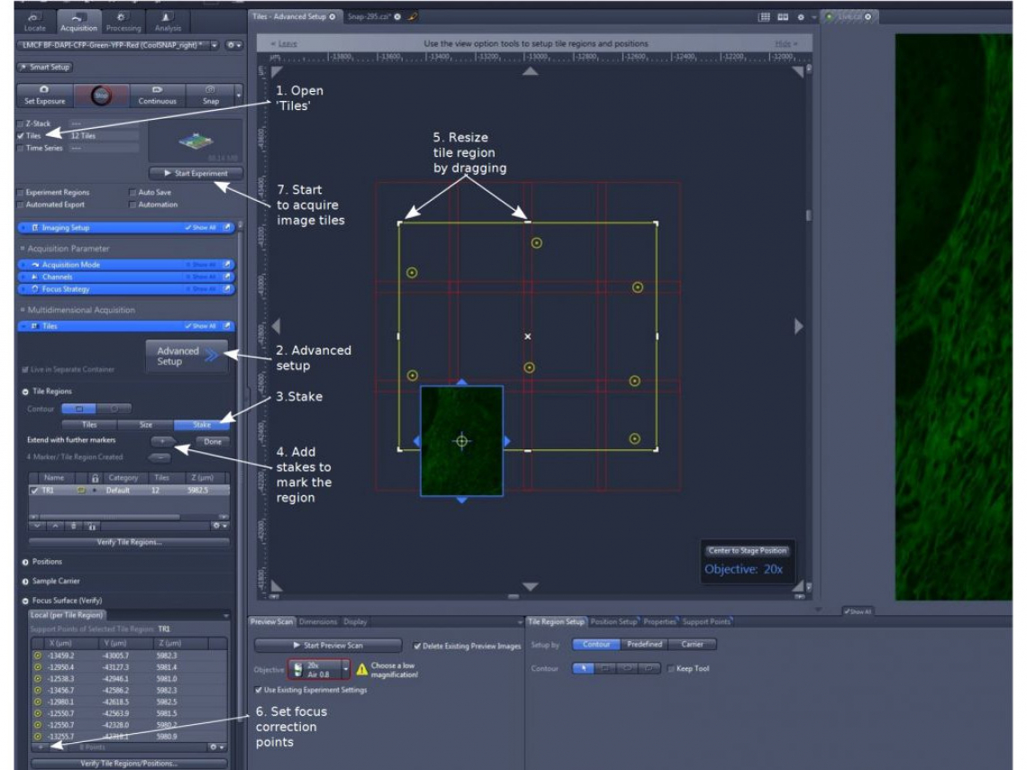
3. 'Focus Surface' setup: This is to set up focus-correction points that allows the user to manually set focuses at locations on the tissue section. The purpose is to 'flatten' out possibly uneven surface of the tissue section.
(1). Open 'Focus Surface (Verify)'
(2). Move the stage to a position, adjust focus, and add (using '+' sign) the x, y, and z information in memory (step 6)
(3). Repeat this step for more positions. Make sure the correction points cover the border area of the sample and distribute evenly across the area. Through calculation, the software determines focuses for tiles not marked with focus-correction points.
4. Click 'Start Experiment' (step 7) to initiate tile acquisition
5. Stitch the tiles together (see below)

Part Three: Tile-scanning from a multiwell plate
1. Tick both 'Tiles' and 'Auto Save' (step 1)
2. In 'Auto Save' (step 2), choose the folder that your data will be automatically saved; 'Automatic Sub-Folder' is preferred that the tile images from each well will be saved in separate sub-folders.
3. In 'Tiles', click to open 'Sample Carrier' and 'Select' a multiwell plate template (step 3); Your plate must be calibrated (step 4) before image acquisition. Calibration is to register: (1) the upper-left corner of the plate, and (2) the positions of the 'containters' (i.e. wells). Open 'Calibrate' and follow the calibration wizard to complete the job
4. Click 'Advanced Setup' that splits the image window into a virtual stage and current live image
5. Record the regions (wells):
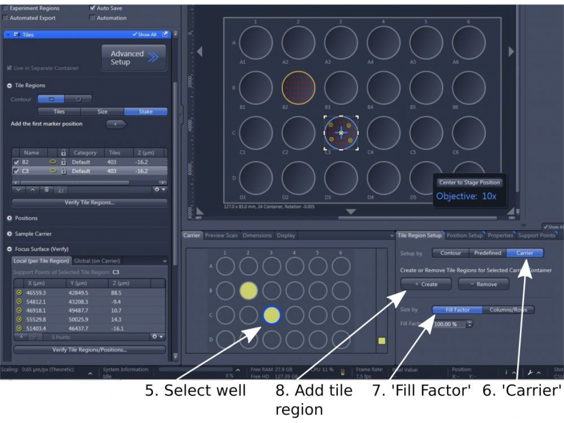
(1). In 'Carrier' near the bottom of the window, double click the well that you wish to image (step 5)
(2). In 'Tile Region Setup', choose 'Carrier' (step 6)
(3) In 'Size By', choose 'Fill Factor' (step 7): 100% to cover the entire well; or other percentage to cover more or less than the entire well; or 'Column x Row' to cover certain area of the well
(4) '+ Create' (step 8) to record the well in the 'Tile Regions'
(5) Repeat (1) to (4) to add other wells to the 'tile regions'
6. Set up focus correction points ('Focus Surface (Verify)'): Double-clicking a well on the screen drives the stage to that well and also highlights the corresponding well in 'Tile Regions'. Focus on the sample, then in 'Focus Surface (Verify)', add ('+' sign) the point (X, Y, and more importantly Z) in memory. It needs at least 4 focus points for the “Focus Surface” to work.
7. 'Start Experiment' to take the images.
8. Stitch the tiles together (see below)
Stitching of Image Tiles:
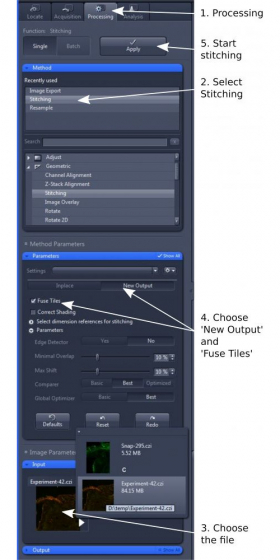
1. Open 'Processing' tab and select 'Stitching' (step 1 and 2)
2. In 'Input', choose the image tiles you wish to stitch (step 3)
3. In 'Parameters', choose 'New Output' and tick 'Fuse Tiles' (step 4). Other parameters are mostly default, but can be adjusted for best alignment and stitching.
4. Click 'Apply' to start the stitching process (step 5). The stitched image will be displayed as a separate image. Please save it in '.czi' format.
1. Contrast adjustment before image export:
For multichannel fluorescent images, the acquired images are shown as channel-merged. 'Split' the channels to display individual channels.

In 'Display', click the channel to be adjusted (step 1), drag the triangles under the histogram for white and black threshold to proper positions (step 2), so that the main structure is lightened up but not oversaturated and the background is dark and clean. Do the contrast adjustment in a sensitive and reasonable manner. Usually, the triangle for black point needs to be positioned right inside the main curve of the histogram. You can also double-click on a channel to have only the channel displayed, then hover the mouse cursor in the background area, read the intensity of the pixels (under 'Pixel Value'), type in the number as the background cut-off value (step 3).
Please keep in mind, adjustment of the contrast only affects the display of the image. It does not change the intrinsic intensity values of pixels in the image.
2. Image Export:
In 'Processing' tab, under 'Method', choose 'Image Export'; In 'Input', choose the image to be exported; In 'Parameters', use TIFF as file type (if a stitched file is too big, JPEG format or resizing the image is also acceptable). If you wish the exported images look as displayed, (for fluorescent images) tick 'Apply display Curve and Channel Color', 'Burn-in Graphics', 'Merged Channels Image', and 'Individual Channels Image' , then 'Apply' to let the image exported. Exporting fluorescent 'Raw Images' is optional.