Andor Dragonfly Spinning Disk Confocal Microscope (User's Manual)

1. Power strip (#1)
2. Spinning disk module (#2)
3. Computer (#3); Login as 'lmcfuser' or using your own account
4. (Optional) Power strip (#4) for heater and CO2 supplying
5. Open Fusion. It is strongly suggested that you refresh the 'Fusion User Data' folder every single time before you start Fusion. That will clean up the settings and possible errors from previous users. Users logged in with their own accounts are also suggested to refresh this folder when they mess up the settings or encounter hard-to-fix problems in the program. This is done in two steps: (1) delete the 'Fusion User Data' folder in 'Documents' folder; (2) Copy/paste back the same-titled folder from the 'BackupDisk' drive. 

A.  Choose an objective:  On the touchscreen display panel of the Leica DMi8 microscope, push ‘Magnification’ icon (1 in Figure 1) to open the control panel. 

1. Push the ‘eye’ icon (2 in Figure 1) to open the port for eyepieces 

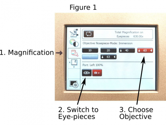
2. Choose the objective (3 in Figure 1) you want to use; Be aware, when you switch between the dry and oil/water objectives, you need an extra push to the objective icon to confirm the choice. Otherwise the objective does not change.

B.  Loading a sample:  Put a sample on the sample adapter. If the objective position is high, lower it down first to avoid scratching of it when loading or moving the sample. Remember, imaging through a #1.5 glass coverglass will ensure you the best image quality.

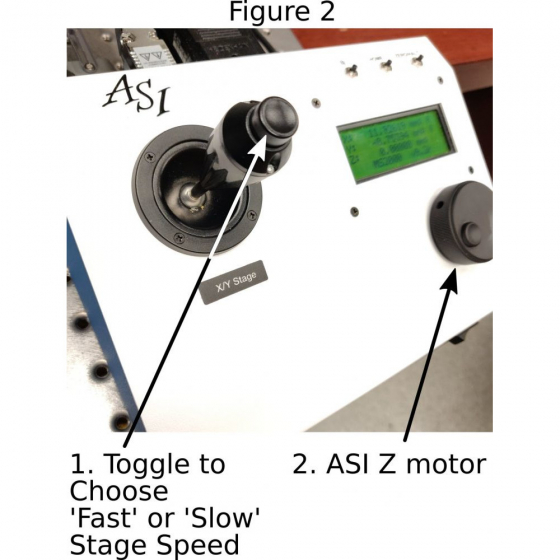
C.  Moving the stage:  Using the joystick on the ASI stage controller to move the stage and position the sample above the objective. Toggle the button on top of the joystick to choose between faster (‘f’ shows on the LCD panel) and slower speeds (‘s’ shows on the LCD panel) (1 in Figure 2).

D.  Using the lights attached to the microscope:  Two LED light controllers are attached to the microscope: one (pE-100) is for viewing samples with bright-field light; the other (pE-300) is for fluorescent samples (three LED lights are available for blue, green, and red fluorescent channels). The two controllers have push-button switches to turn the lights ON or OFF. Light intensity is also adjustable.

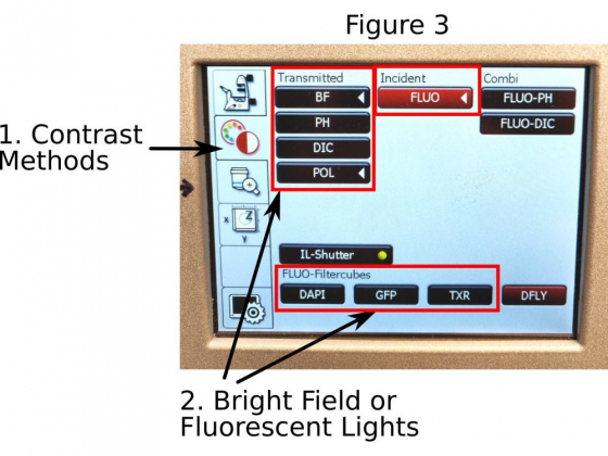
E.  Bright field or fluorescence:  Push the ‘Contrast Methods’ icon (1 in Figure 3) on the touchscreen to open the page. BF, Ph, and DIC are for bright-field illumination; For best bright-field contrast, you also need to manually select a filter in the condenser to match the objective used; Selections for the DAPI, GFP, and TxRed filter cubes are for blue, green, and red fluorescent channels separately.

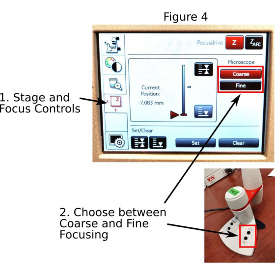
F.  Focusing:  The focus knobs on the microscope move the objective in faster (bigger knob) or slower (smaller knob) speed. On the Leica touchscreen open ‘stage and focus controls’ panel (1 in Figure 4) where you can further set up the focus knobs in ‘coarse’ or ‘fine’ modes (2 in Figure 4). Be alert that most of the objectives on the microscope have very short working distances. It is important to avoid crashing of the objective with the sample.

A Leica SmartMove is connected to the microscope for focusing as well. The ‘coarse’ or ‘fine’ modes can also be activated by buttons on the Leica SmartMove (2 in Figure 4).

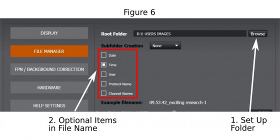
A.  Fusion saves an image (or serial of images in multidimensional acquisition modes) automatically. Therefore, you need first to set up a folder on the local hard drives (preferably) and a file name for your image.

A basic image name should be given (1 in Figure 5). Click on the icon ‘…’ (2 in Figure 5) to open the ‘File Manager’ where to set up the folder (1 in Figure 6) and to complete the file name by optionally adding imaging date, time, channel name, or protocol label (2 in Figure 6) that are appendices to the basic image name. Then return to imaging window.

B.  Open the triangle on the right side of Fusion window (3 of Figure 5) to expand the work area.

‘Channel Manager’ tab is displayed. However, users are not recommended to make changes in here before they know how the system works. Changes on many items in ‘Channel Manager’ will be remembered by the system and are carried on to future experiments. LMCF provides a basic channel setup included in the 'Fusion User Data' for users to start with.

C.  Instead, open ‘Protocol Manager’ tab (step 1 in Figure 7) to set up a protocol: for image acquisition in combinations of single/multiple channels, time lapse, z-stacks, multiple positions, montage acquisition (tile scanning and stitching), and hardware autofocusing

1. Set up channels and single point image acquisition:

   

    

(1)   Open ‘Protocol Manager’, click ‘New Protocol’, and name it (2 in Figure 7)

(2)   LMCF channel settings are grouped in ‘CF25’, ‘CF40’, ‘TIRF’, ‘DIC’, ‘Dual Channel Acquisition’, DIC for CF25, DIC for CF40, and etc. In general, for the 10x and 20x dry objective lenses, the settings under ‘CF25 (confocal with 25um pinhole size)’ should be used while settings under ‘CF40 (confocal with 40um pinhole size)’ should be used for the 40x oil, 63x oil, 100x oil and the 63x water immersion objective lenses.

(3)   Select channels from the preset channel pool and add them to the protocol (3 in Figure 7). It is suggested that the same camera is used for channels in one protocol.

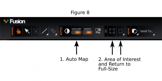
(4)   Activate ‘Auto Map’(1 in Figure 8)

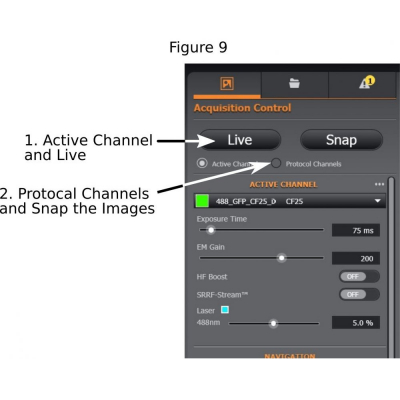
(5)   Finding good exposure for each channel: Use ‘Active Channel’, start ‘Live’ mode (step 1 in Figure 9), adjust exposure time, laser intensity, and EM gain if the EMCCD camera is used (EM Gain at 200 is suggested);

Never set up those exposure parameters based on the display of the images; Rather, you need to read the fluorescent intensities from the structure of interest and from the background by hovering the cursor over them. In general, at least 3 times (the higher the better) difference in intensity between them is desired for publication quality images.

In the Camera section in Channel Manager, the cameras can be set to take multiple images ('Frame Averaging') and the images are averaged to generate a 'cleaner' image; For the iXon EMCCD camera, 'Symmetrical Binning' can increase the camera sensitivity and image contrast, but at the cost of lower resolution of the images.

(6)  Tick ‘Protocol Channels’ and ‘Snap’ the images (step 2 of Figure 9).

2. Set up and acquire multi-dimensional acquisition (you may only need some of the following functions)

(1)  Time Repeats:

(a) Time interval: The time between the starts of two consecutive acquisitions; For single point acquisition, it is ‘1’.

(b) Total time points or total time period of experiment: These two parameters are linked to each other. Changing one also changes the other.

(2)  Focus Stabilization (hardware autofocusing): Start the function by ticking ‘Draft Stabilization Enabled’ (better to choose stabilization for ‘All Fields’) and by ticking ‘Draft Stabilization Mirror Inserted’. Both items have to be activated or inactivated together. Otherwise the system will report error.

(3)  Multi-Field Positions: That is to add multiple imaging positions in the sample. In a time-lapse acquisition, those positions will be re-visited at each time point. Adding (‘+’) a position in the list allows the system to memorize its coordinates and focus (x,y,z), as well as the autofocus offsets. The saved positions can be deleted, refreshed, or re-ordered.

(4)  Z Scan Settings:

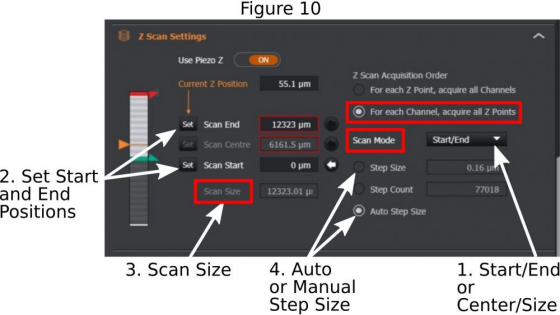
(a)  Z stack range: For multi-field position acquisition, use ‘center/range’ method in ‘Scan Mode’ (1 in Figure 10); Add a ‘Scan Size’ in micrometers (in Figure 10); The system will mark the current focus as the center point of the entire z-stack. For single field acquisition, you may use ‘Start/End’ method in the ‘Scan Mode’; Use the ASI piezo Z (2 in Figure 2) to find one end of the future z-stack, set ‘Scan Start’ (2 in Figure 10); Then find another end of the z-stack and set ’Scan End’;

(b)  Step size: Choose  ‘Auto Step Size’  (4 in Figure 10) if the future z-stacks will be used for 3-D reconstruction or deconvolution; But if you plan to do maximum intensity projection of the z-stacks, a step size that is about 4x-6x of the ‘Auto Step Size’ may be entered.

(c)  For fixed samples, it is better to choose ‘For each Channel, acquire all Z points’

(5)   Montage: This is a tile-scanning and image-stitching procedure. There are two ways to set up the scanning area (the future area will be a rectangle in either way):

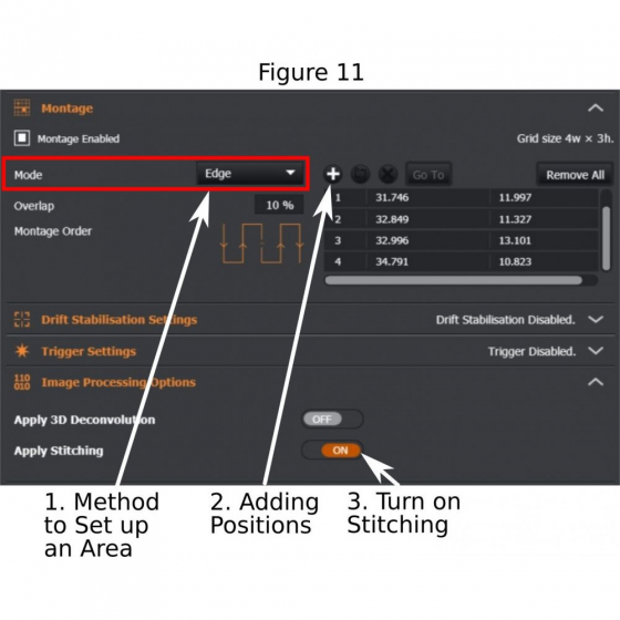
(a) Mode – ‘Tiles’ (1 in Figure 11): input numbers of tiles in x and y axis;

(b) Mode – ‘Edge’ (1 in Figure 11): Start ‘Live’, move the stage to identify the edges of the sample, and add (2 in Figure 11) those edges to the list. A minimum of two edge positions are required for ‘Montage’ to work. If more edge positions are added, the system will draw a rectangular area to cover the furthest points.

(c) In ‘Image Procession Options’, tick ‘Apply Stitching’ (3 in Figure 11); A single image of stitched tiles will be produced after the tile-scanning is completed.

(d) It is known that the illumination in the field is not uniform, especially it is weaker near the borders. To mitigate the artifacts (mainly visible ‘seams’ between fused tiles in the final stitched image), the central area of the camera chip may be cropped (2 in Figure 8) and used for 'Montage'.

(6)   Click ‘Acquire’ to start a multi-dimensional acquisition.

D.   Acquired images in Fusion may be opened in Imaris, ImageJ, or Fiji for further processing.

Super-Resolution Radial Fluctuations (SRRF, pronounced as ‘surf’) :

1.  Use the 63x oil or 100x oil objective to achieve the best resolution

2.  Set up a protocol that uses the iXon EMCCD camera

3.  Set image acquisition at 2x magnification for the EMCCD camera

4.  Choose a small region (ROI: region of interest, see 2 in Figure 8) for fast imaging

5.  Use a short exposure time (for example less than 50 ms). Loss in fluorescent intensity due to the short exposure time can be compensated by increasing the laser power. But make sure the structure of interest is not oversaturated. As a matter of fact, relatively lower fluorescent intensity generates better SRRF images with less artifacts in Fusion.

6.  Turn on ‘SRRF-Stream’ (in Channel Manager and under 'iXon EMCCD camera')

7.  Set ‘SRRF Frame Count’ between 50-150;  ‘SRRF Radiality Magnification’ to 4x;  ‘SRRF Ring Radius’ to around 1 (a smaller ring radius produces better resolution, but is prone to more artifacts); Use ‘mean’ for ’SRRF temporal Analysis’

8.  Click ‘Snap’ for single SRRF image acquisition; Or click ‘Acquire’ for multidimensional image acquisition with SRRF.

A.   Lower down the objective and very gently wipe off the oil or water if an oil or water objective has been used;

B.   Check the online booking calendar and

1.  If next user comes to use the microscope in one hour, close Fusion, and leave the system on;

2.  If nobody will use it in the next hour, turn off the heater if it has been used (switch #4), close Fusion and shut down the computer (switch #3), switch off #2 and #1.